Olist Data Analysis

Project Overview

This project explores the Olist dataset (the largest department store in Brazilian marketplaces) to uncover hidden patterns in sales performance, customer geography, and product profitability.
Facing a dataset of almost 100,000 orders spanning multiple tables and relationships, the goal was to build a scalable relational structure and extract high-level KPIs to drive executive decision-making.

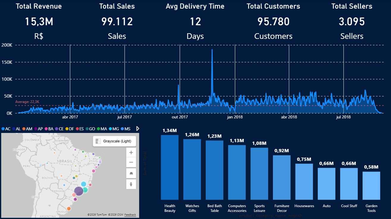
Executive Overview

This panel provides a granular day-to-day view of the marketplace operation, highlighting daily volatility in sales and logistics.
Beyond temporal trends, it integrates geospatial distribution to identify regional clusters and a categorical breakdown to pinpoint the top-performing product niches. All metrics summarize 100k+ records through optimized SQL (detailed here).

Core Technologies

• PostgreSQL: Advanced query optimization, CTEs, and Window Functions.
• Relational Database Design: Data Polishing and Normalization with Entity-Relationship modeling.
• Power BI & CSV Analytics: Data visualization with Business Intelligence & Storytelling.

The Challenge

Re-establishing a database structure within PostgreSQL and transforming it into structured environment capable of answering complex business questions.
Such as:

• How is the business performing over time?
• Which categories have the highest product prices?
• Which product categories contribute most to total profit?
• How are the categories distributed in percentage?
• Where are the best places for distribution centers?
• How does customer distribution vary across regions?

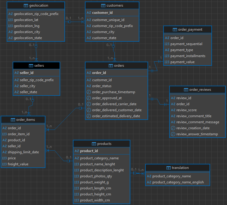
Strategic Architecture

Everything should start with a solid foundation, as such, the first step was mapping the entity relationships to ensure that every join across the 100k+ orders remained accurate and efficient.
Below is the normalized database schema designed to ensure data integrity and optimized retrieval.

Entity Relationship Diagram

Queries

• Query 1 - How is the business performing over time?

  Description:

  Calculates daily revenue and computes a weekly average.

  SQL Code:

  With daily_revenue as (
      SELECT SUM(oi.price) AS revenue,
          o.order_approved_at::date AS p_date
      FROM orders o   
          JOIN order_items oi ON o.order_id = oi.order_id
      GROUP BY p_date
      )
  
  SELECT p_date, revenue,
      ROUND(AVG(revenue) OVER 
      (ORDER BY p_date ROWS BETWEEN 6 PRECEDING AND CURRENT ROW)::numeric, 2) AS weekly_avg
  FROM daily_revenue;

  Results:

  

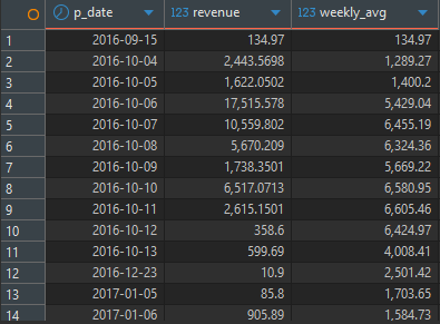
  Note: Profit calculations are based on available dataset attributes and do not include operational costs beyond freight.

  Insight:

  Analyzing the weekly moving average allows for smoothing out daily fluctuations and identifying the true growth or decline trends in sales by eliminating noise from isolated peaks.

  Business Value:

  It assists the planning team in forecasting inventory and staffing needs based on medium-term trends rather than just the previous day's performance.

  Visualization:

  The following graph illustrates the monthly revenue, helping to identify historical patterns and business evolution.

  

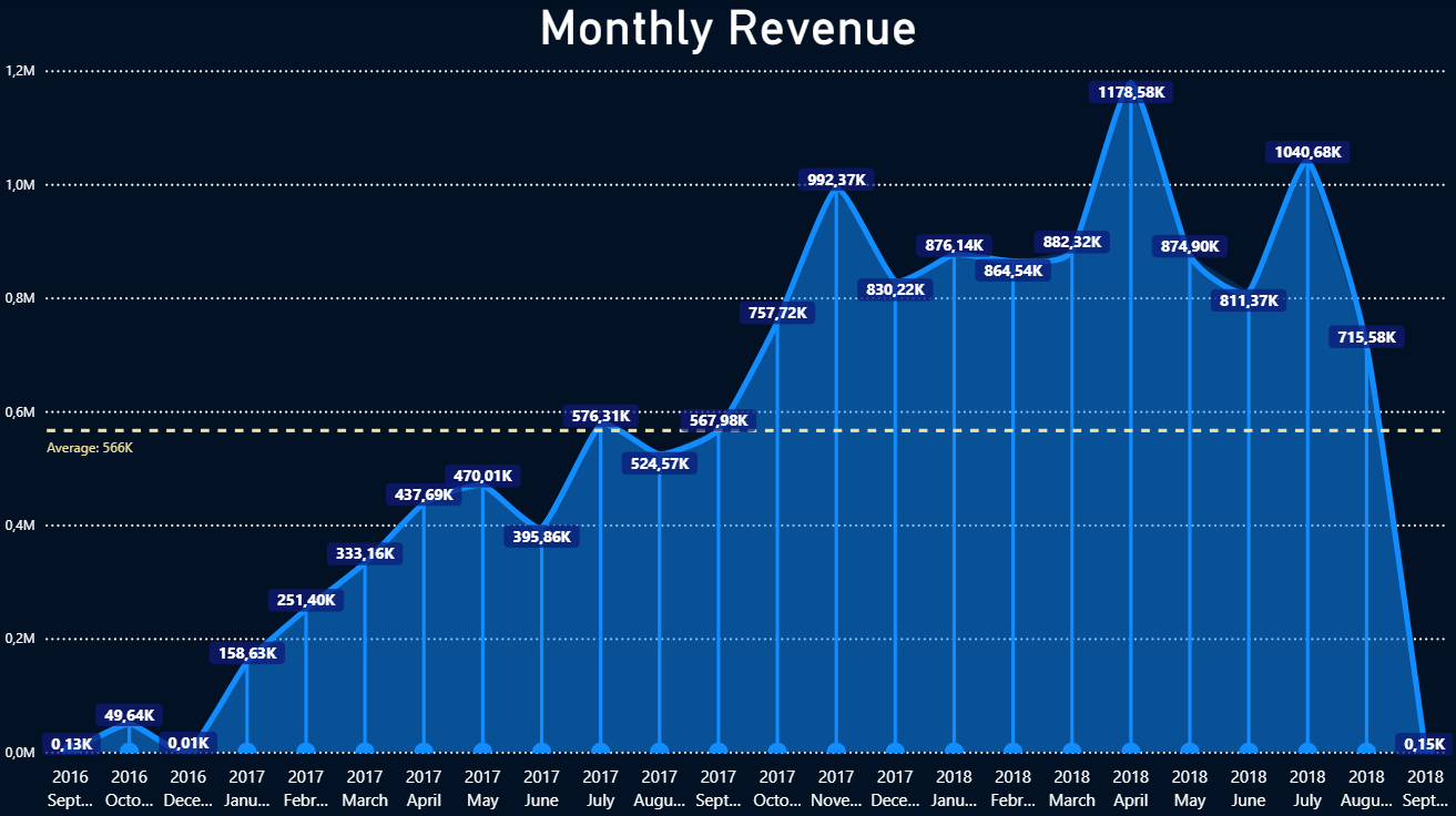
  Graph made with CSV created from the query results.

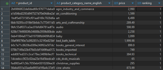
• Query 2 - Which categories have the highest product prices?

  Description:

  Ranks products within each category based on their prices.

  SQL Code:

  SELECT DISTINCT t.product_category_name_english AS Category,
      oi.price AS Price,
      DENSE_RANK() OVER (PARTITION BY p.product_category_name ORDER BY oi.price DESC) AS Ranking
  FROM products p 
      JOIN order_items oi ON p.product_id = oi.product_id 
      JOIN "translation" t ON p.product_category_name = t.product_category_name
  ORDER BY oi.price DESC, ranking ASC, t.product_category_name_english;

  Results:

  

  Insight:

  By using DENSE_RANK, it is possible to identify "premium" (high-end) products within each segment without skipping positions in the classification.

  Business Value:

  Enables the marketing team to create targeted campaigns for "Luxury/Premium" audiences within specific categories.

  Visualization:

  The following graph illustrates categories that have pricier products.

  

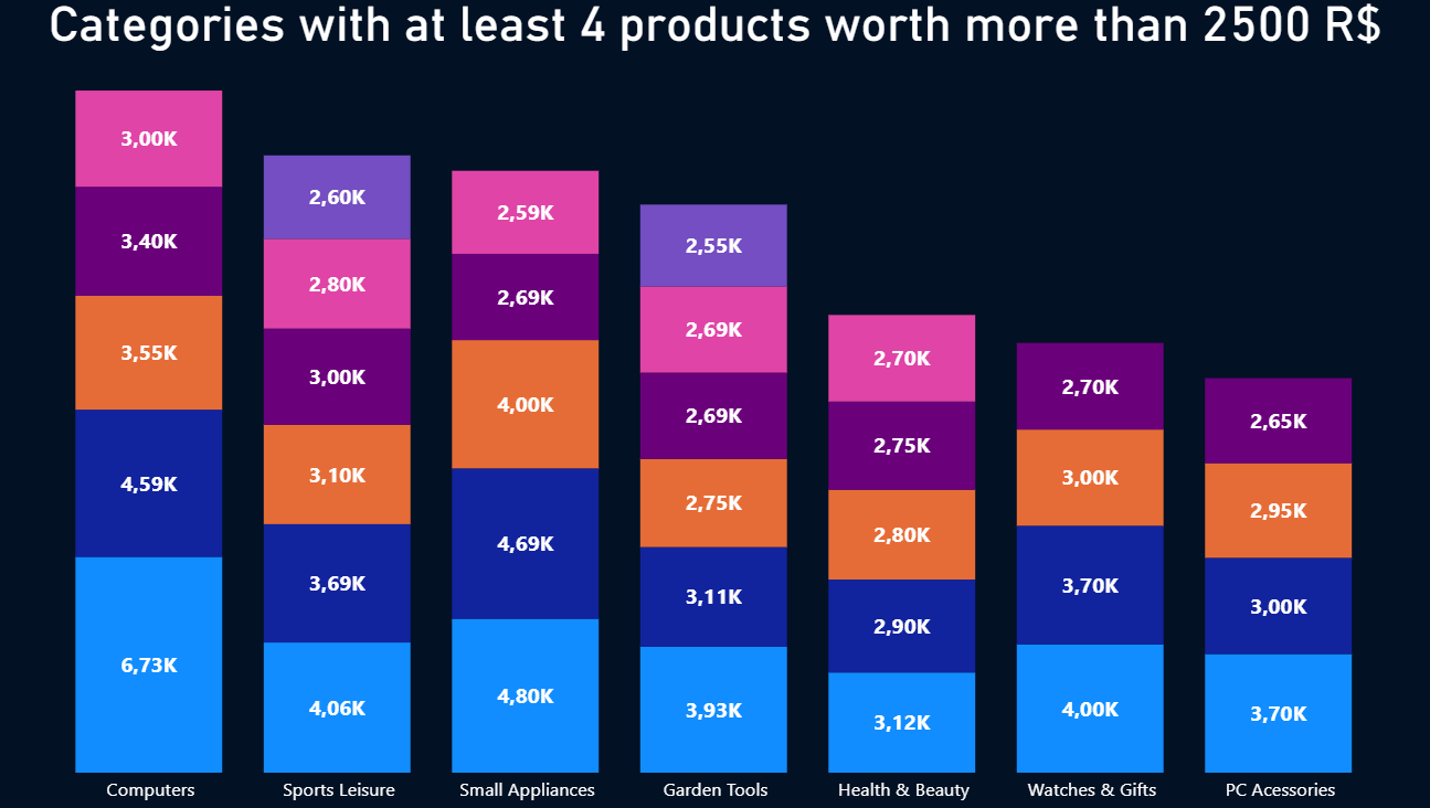
  Graph made with CSV created from the query results.

• Query 3 - Which product categories contribute most to total profit?

  Description:

  Retrieves the top 5 product categories that have generated the highest total profit.

  SQL Code:

  SELECT t.product_category_name_english AS category,
      ROUND(SUM(oi.price * oi.order_item_id)) AS income
  FROM products p 
      JOIN order_items oi ON p.product_id = oi.product_id 
      JOIN translation t ON p.product_category_name = t.product_category_name 
  GROUP BY t.product_category_name_english 
  ORDER BY income DESC
  LIMIT 5;

  Results:

  

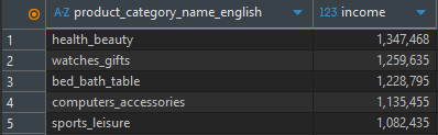
  Insight:

  Identifies the primary revenue drivers for the company. Categories such as Health & Beauty and Watches & Gifts emerge as leaders, accounting for a significant portion of total profit.

  Business Value:

  Directs investment in advertising and partnerships toward the categories that yield the highest direct return on investment (ROI).

  Visualization:

  The following graph illustrates the top 5 most profitable categories.

  

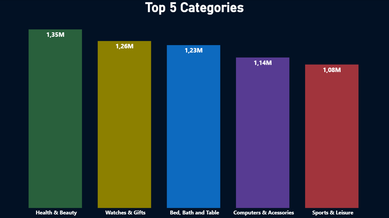
  Graph made with CSV created from the query results.

• Query 4 - How are the categories distributed in percentage?

  Description:

  Calculates the percentage contribution of each product category to the total income.

  SQL Code:

  WITH income_pct AS (
  SELECT t.product_category_name_english AS category,
      ROUND(((SUM(oi.price) / SUM(SUM(oi.price)) OVER())::NUMERIC * 100),2) AS pct
  FROM order_items oi 
      JOIN products p ON oi.product_id = p.product_id 
      JOIN "translation" t ON p.product_category_name = t.product_category_name 
  GROUP BY t.product_category_name_english)
  
  SELECT * FROM income_pct
  WHERE pct > 0
  ORDER BY pct DESC;

  Results:

  

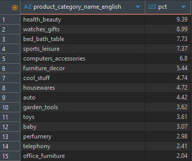
  Insight:

  This Pareto-style analysis reveals that the top categories represent a disproportionate percentage of total income, often following the 80/20 rule where a small group of products generates most of the revenue.

  Business Value:

  Critical for merchandising decisions and inventory management, as it highlights which categories to prioritize, it is also helpful for understanding the company's dependency on specific market niches.

  Visualization:

  The following graph illustrates the percentage of total income contributed by each product category.

  

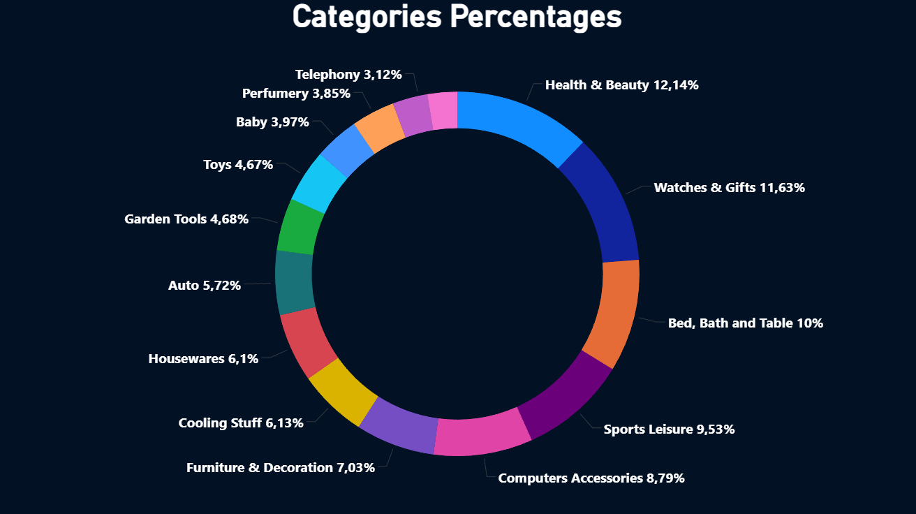
  Graph made with CSV created from the query results.

• Query 5 - Where are the best places for distribution centers?

  Description:

  Ranks cities based on the number of customers in each city.

  SQL Code:

  SELECT g.geolocation_city || ',' || g.geolocation_state || ',' || 'Brasil' AS geolocation,
      COUNT(c.customer_city)
  FROM customers c 
      JOIN geolocation g ON c.customer_zip_code_prefix = g.geolocation_zip_code_prefix 
  GROUP BY g.geolocation_city ,g.geolocation_state
  ORDER BY COUNT(c.customer_city) DESC;

  Results:

  

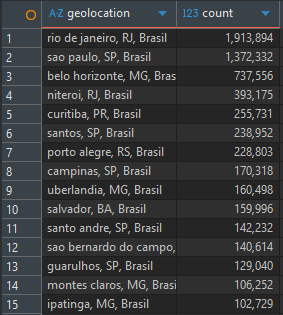
  Insight:

  Customer volume is heavily concentrated in major hubs like Rio de Janeiro, São Paulo, and Belo Horizonte. As such, these cities are ideal locations for distribution centers.

  Business Value:

  Guides logistics strategies, such as establishing distribution centers (hubs) near these clusters to reduce delivery times and shipping costs (freight).

  Visualization:

  The following map shows the 15 cities with the highest customer counts.

  

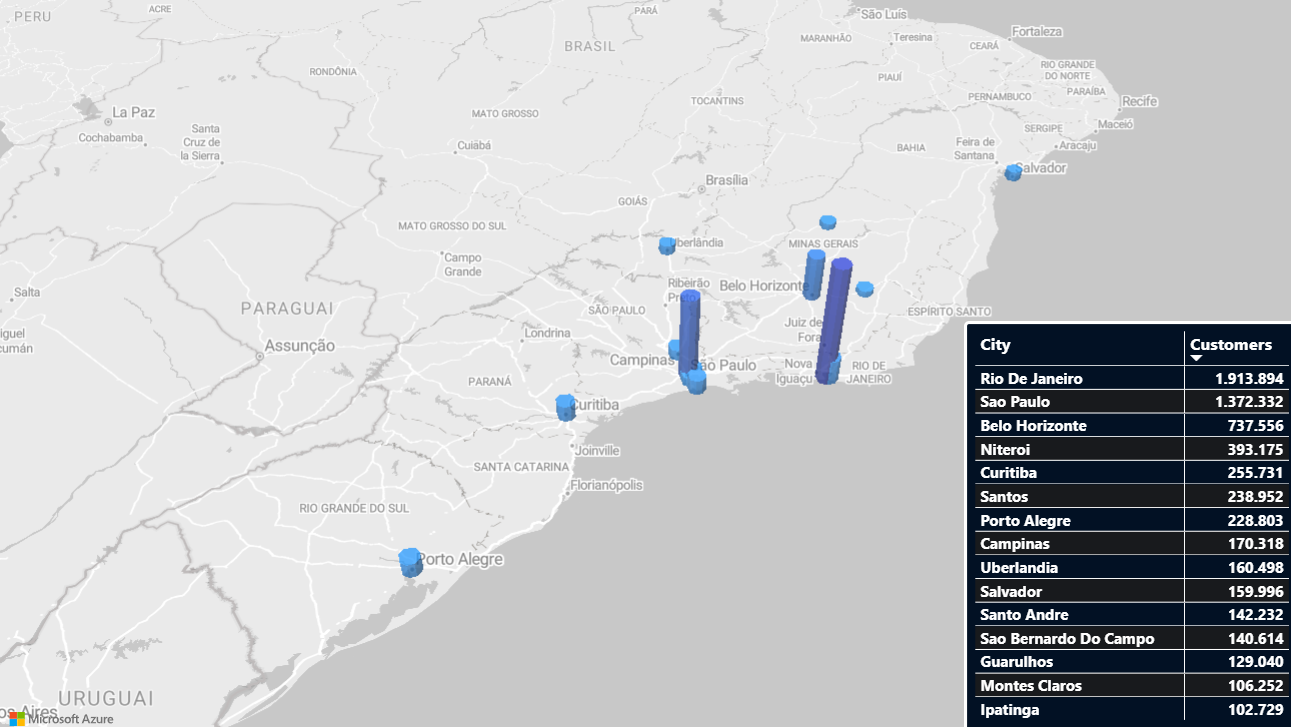
  Graph made with CSV created from the query results.

• Query 6 - How does customer distribution vary across regions?

  Description:

  Ranks Brazilian states based on the number of customers in each state.

  SQL Code:

  SELECT g.geolocation_state, 
      COUNT(c.customer_state) 
  FROM customers c 
      JOIN geolocation g on c.customer_zip_code_prefix = g.geolocation_zip_code_prefix 
  GROUP BY g.geolocation_state
  ORDER BY COUNT(c.customer_state) DESC;

  Results:

  

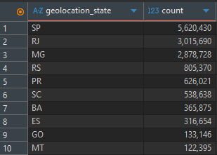
  Insight:

  The state of São Paulo (SP) leads by a significant margin, followed by RJ and MG, solidifying the Southeast region as the primary consumer market.

  Business Value:

  Allows for personalized regional promotions and provides insights into brand penetration in states with lower customer representation, such as MT and GO, where there is growth potential.

  Visualization:

  The following map illustrates the customer distribution across Brazilian states.

  

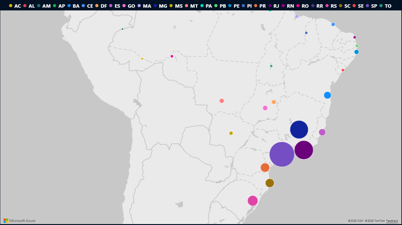
  Graph made with CSV created from the query results.